Time in Machine Learning Engineering ⏳

Time in Machine Learning Engineering ⏳ - A Faux-Calculus Argument

This article started out as a joke and didn’t wander very far in state space. It is a witty and not-so-rigorous attempt to demonstrate the importance of time in ML projects that will annoy most mathematicians and alienate some physicists. There’s some truth in it… it’s just really hard to find. Enjoy! 😛

Update: This article is now available on Medium

Time in Software Engineering

There’s a saying at Google about software engineering (SWE, for short) that goes something like this (Winters, Manshreck & Wright, 2020):

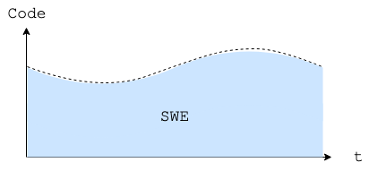
"Software engineering is programming integrated over time."

Now, in case you don’t know this about me, I love taking things too literally and seeing how far I can go - that’s just how I roll, with utter disregard for the consequences of my deductions and derivations. Consider yourself warned! ⚠️

We can represent the assertion above in a nice, compact way using a simple formula

\texttt{SWE} ~=~ \int \texttt{Programming} ~dt

The original quote doesn’t specify start and end values for the integration, so we’ll leave it indefinite for now.

For lack of a better name, I’ll call this method of using calculus (or something close to it) to represent catchy slogans and witty remarks “Faux Calculus”.

The late Patrick Winston using faux-calculus while delivering his annual talk on 'How to Speak' - an MIT tradition for over 40 years

If there’s one key insight we can take from all of this is that SWE is more than just writing code – it’s about maintaining that code over time.

In fact, engineering in general is mostly about creating things that will stand the test of time. We often use expressions like “future-proof”, “long-term” and “reliable” to stress how important it is to build lasting solutions.

In that sense, engineering can be described as a functional (high-order operator, in CS terms) that integrates whatever you’re building over time

$f \mapsto \texttt{E}[f] = \int f ~dt$

Using a postfix notation, this can be represented as $f\texttt{E}$ - so that $\texttt{SWE}$ is really just $\texttt{E}[\texttt{SW}]$ .

“Ok” I hear you say “These formulas are cool and all” (if you’re a working mathematician, you’re probably shouting at the screen and pulling your own hair at this point) “But why are we making such a big fuss about time? What makes it so important?”

Well, I’m glad you asked!

In case you haven’t noticed, time changes everything ⌛ (Just read Percy Bysshe Shelley poem Ozymandias!)

"My name is Ozymandias, King of Kings; / Look on my Works, ye Mighty, and despair! / Nothing beside remains. Round the decay / Of that colossal Wreck, boundless and bare / The lone and level sands stretch far away."

In the world of SW development, the effects of the passage of time are especially dire:

Developers come and go
Programming languages go out of style
Frameworks go out of date
Features turn old and obsolete (or worse, irrelevant)
Code begets legacy code
Documentation… well, don’t get me started on documentation.

According to platonic lore, the pre-socratic philosopher Heraclitus (AKA the weeping philosopher 😭) was one of the first to propose the idea that change is the only constant in the Universe (Πάντα ῥεῖ).

In this constant flow of change (pun intended), the only solutions that thrive and prosper are the ones that react and adapt to change in a timely manner.

The ones that don’t, the ones that choose the easy way, the “road most traveled”, start to accrue debt… of the technical kind.

Don’t you just love a good economical metaphor, dear reader? 📈

Unlike the Graeberian notion of debt as a “perversion of a promise” (Graeber, 2011), technical debt is non-negotiable. If a project intends to keep the proverbial lights on, it needs to be repaid… in full (*). This entails keeping up with all the “promises” made by the PM to the stakeholders when writing the project charter and by the SW engineers when documenting their code.

(*) There’s also the vaguely keynesian “keep throwing spaghetti at the wall until it sticks” approach - as long as the headcount is strictly increasing and the technical debt per capita is decreasing, we should be fine. The Mythical Man-Month crew probably wouldn’t agree with this. But, to be honest, when it comes to finding economical solutions to technical debt, there are probably goats behind every door 🚪 $\rightarrow$ 🐐.

Dilbert on the old 'keep throwing spaghetti at the wall until it sticks' approach

Time in Machine Learning Engineering

It probably won’t come as a surprise that ML projects are also prone to technical debt.

However, and therein lies the big difference to vanilla SW projects: much like cultural onions 🧅 and icebergs 🧊 or the dark sector of our Universe 🌌, most of this debt is just lurking behind the scenes, virtually invisible to uninitiated and untrained eyes.

In a paper presented at NeurIPS, provocatively titled “Hidden Technical Debt in Machine Learning Systems” (AKA “Machine Learning: The High Interest Credit Card of Technical Debt” 💳), Sculley et al. (2015) argued that there are no “quick wins” in real-world ML systems and that nothing ever comes for “free”.

Their simple representation of a ML system as a disjoint set of “boxes” is probably one of the most iconic and used images in the whole ML Operations (MLOps) literature. And for good reasons.

Real-world ML systems are more than just ML code (Sculley *et al.*, 2015)

It illustrates two very important yet often dismissed facts about real-world ML:

1/ How complex ML development can be and

2/ How small the “cool stuff” (ML code) is compared to everything else AKA “plumbing” (data, infrastructure, &c.).

Failing to acknowledge either 1 or 2 and their consequences will lead any promising ML endeavor to spiral out of control and crash. According to a recent Gartner report, around 90% of all AI and ML projects fail to deliver (!), and only half of them ever make it to production (!!!).

Can we reverse this tendency? Something needs to change… but what?

In the remainder of this article, I’ll argue, using the same faux-calculus reasoning we applied to SWE, that ML practitioners everywhere should handle time more carefully, and explore what that means for Machine Learning Engineering (MLE).

Let’s start with the basics…

Nowadays, when delivering an ML 101 presentation, it has become standard practice to include a slide comparing traditional programming and ML, with strong claims about how much of a ‘paradigm shift’ it is to go from one to the other (Thomas Kuhn is probably rolling in his grave 🪦).

This often translates to something along the lines of

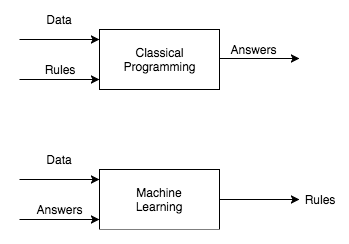
ML vs Traditional Programming (source: O'Reilly)

or, focusing only on the ML portion

These are often abbreviated as

$\texttt{ML} ~=~ \texttt{Code} + \texttt{Data}$

For most ML applications, however, this picture is too simplistic.

A better alternative, put forward in Martin Fowler’s Continuous Delivery for ML (CD4ML) article, involves the notion of 3 axis of change

Martin Fowler's 3 axis of change - Data, Model and Code

which can be summarized as

$\texttt{ML} ~=~ \texttt{Code} + \texttt{Data} + \texttt{Model}$

You probably see where I’m going with this, right?

Let’s apply the engineering ( $\texttt{E}$ ) operator to our new definition

$\texttt{MLE} ~=~ \int \texttt{Code} + \texttt{Data} + \texttt{Model} ~dt$

We can translate this into something more readable

MLE is just a bunch of stuff summed up together, integrated over time

Sounds ominous, doesn’t it? Too bad it’s dead wrong!

As any freshman calculus student knows (integration-wise, that’s probably the only thing most of them know by the time they graduate), the sum rule of Integration tells us that

The integral of the sum is the sum of the integrals

Differentiation vs Integration (source: xkcd)

So, in simple terms, our formula is just telling us that

$\texttt{MLE} ~=~ \int \texttt{Code} ~dt + \int \texttt{Data} ~dt + \int \texttt{Model} ~dt$

If we equate $\texttt{Code}$ with $\texttt{Programming}$ (which is debatable to be sure, but let’s keep with it for now), then we’re basically saying that

MLE is just good old SWE, data engineering and something we don't yet know what to call or how to handle, summed up together

which is a gross oversimplification.

By the way, just in case you’re wondering about this, I’m assuming that every term in that integral has an explicit time dependence.

Schematically, this can be represented as

$\texttt{Data} ~=~ \texttt{Data}(t)$

$\texttt{Model} ~=~ \texttt{Model}(t)$

$\texttt{Code} ~=~ \texttt{Code}(t)$

If this were not the case, then each one of these “terms”, at least w. r. t. time, would be a trivial matter to solve.

So what’s wrong with this line of reasoning? And how, if at all, can we fix it?

There are two main issues with our initial approach.

The first is that the definitions above don’t really take into account the close dependencies between the 3 axis of change.

Interdependencies between the 3 axis of change

$\texttt{Model}$ relies heavily on the quality of the $\texttt{Data}$ used for training, validation and testing - the old “Garbage In, Garbage Out” (GIGO) dictum.

On the other hand, $\texttt{Code}$ needs to adapt both to the $\texttt{Model}$ used for inference and the $\texttt{Data}$ that is fed into it.

In faux calculus, we can easily represent these relations by adding a few arguments

$\texttt{Data} ~=~ \texttt{Data}(t)$

$\texttt{Model} ~=~ \texttt{Model}(\texttt{Data}, t)$

$\texttt{Code} ~=~ \texttt{Code}(\texttt{Data}, \texttt{Model}, t)$

The question of whether $\texttt{Model}$ depends explicitly on time is a matter of philosophical debate.

Making copious use of the chain rule, we can start asking some deep questions about any ML system:

1/ How does the $\texttt{Data}$ change over time?

$\frac{d~\texttt{Data}}{d t}$

And, if you’re feeling fanciful, if $(X, y)$ is a dataset containing input variables $X$ and target values $y$ , how can we distinguish data drift ( $X$ changes) from concept drift ( $X \rightarrow y$ changes) within the faux calculus framework (Quiñonero-Candela et al., 2009)?

2/ Is there an effective way to deal with $\texttt{Model}$ drift?

$\frac{d~\texttt{Model}}{d t} = \frac{\partial~\texttt{Model}}{\partial~\texttt{Data}} \frac{d~\texttt{Data}}{d t} + \frac{\partial~\texttt{Model}}{\partial t}$

3/ Can $\texttt{Code}$ be decoupled from $\texttt{Model}$ changes?

$\frac{d~\texttt{Code}}{d t} = \frac{\partial~\texttt{Code}}{\partial~\texttt{Data}} \frac{d~\texttt{Data}}{d t} + \cancel{\frac{\partial~\texttt{Code}}{\partial~\texttt{Model}}} \frac{d~\texttt{Model}}{d t} + \frac{\partial~\texttt{Code}}{\partial t}$

Finally, there’s the (erroneous) assumption that we can just sum everything up and call it a day.

As any ML engineer will tell you, reality is probably closer to something like this

$\texttt{MLE} ~=~ \int^{EOL}_{idea} L(\texttt{Data}, \texttt{Model}, \texttt{Code}, \texttt{Data}', \texttt{Model}', \texttt{Code}', t) ~dt$

where the prime (‘) represents a derivative w.r.t. time and $EOL$ (end-of-life) indicates the inevitable demise of the ML system - hopefully, at a point far into the future.

Using Winstonian notation, we can easily produce a data-centric version - why is it or is it not true that we spend most of our time in or around data?

$\texttt{MLE} ~=~ \int^{EOL}_{idea} L({\huge\texttt{Data}}, {\tiny\texttt{Model}}, \texttt{Code}, {\huge\texttt{Data}'}, {\tiny\texttt{Model}'}, \texttt{Code}', t) ~dt$

If you’re seeing 80/20 patterns everywhere, you may be suffering from **Paretolia** - a pareidolic tendency to see instances of Pareto’s principle where there are none — please consult your physician for personalized medical advice ⚕️ (source: Forbes)

The $L$ function is mostly problem- and system-dependent, and it’s actual form is usually unknown - sometimes even unknowable.

The takeaway message, if there’s one, is that the dynamics of applying engineering principles to ML systems of any kind is something really tricky (Paleyes, Urma & Lawrence, 2020), not to be trifled with.

Mind you, some problems do have solutions (Lakshmanan, Robinson & Munn, 2021), but those only cover edge cases and require reading a bunch of O RLY books.

An example of an MLE lifecycle (Burkov, 2020)

If you’re a physics nerd like me, you probably noticed that I called that function $L$ (*nudge *nudge *wink *wink).

Without getting into variational calculus (which is probably well beyond the scope of this essay) or defining exactly what $L$ is (pssst, it involves the kinetic and potential energies of the ML system, whatever those are), then there seems to be a link between the Principle of Stationary Action

$\delta S = 0$